Finding Ships in Radar, Without a Neural Net

Draw a box over water, pick a Sentinel-1 pass, and get every ship in it as a marker with a measured length, beam, heading, and a cargo / military / other call. It runs entirely on your own machine, needs no account anywhere, and tells you when it isn't sure.

The accuracy is 71% on type, measured against AIS ground truth. That number started at 56%. Getting from one to the other is what this tutorial is about.

Why radar instead of a photograph

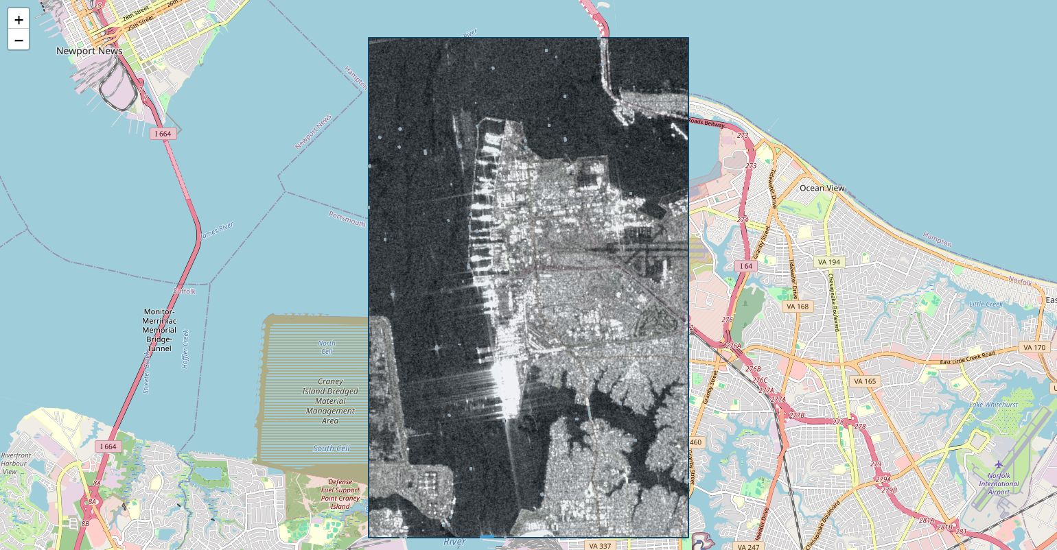
Optical satellites need daylight and a hole in the clouds. Synthetic aperture radar needs neither, which is the entire reason it exists. A ship is a corner reflector sitting on a surface that scatters almost nothing back, so vessels show up as bright points on a dark field. That contrast is the whole detection problem, and it is why this works without machine learning.

The data source is Microsoft Planetary Computer's sentinel-1-rtc collection. It is anonymous, 10 metre, north-up UTM, and cloud-optimised. The alternatives all fail on access rather than quality: earth-search's GRD bucket is requester-pays, Copernicus Data Space wants an account and enforces quota, and ASF wants an Earthdata login. RTC's real limit is that it is only processed where a terrain model exists, so there is no mid-ocean coverage. That does not matter. Ships are in ports and straits.

Detection is CFAR

Constant false alarm rate detection compares each pixel to the statistics of the water around it rather than to a fixed brightness. A pixel is a candidate when it exceeds its own local background by enough that the odds of speckle producing it are below your tolerance.

# Local mean and variance from integral images, then a per-pixel threshold.
mean, var = local_stats(img, guard=7, window=31)
threshold = mean + k * np.sqrt(var)
candidates = img > threshold

The trap is memory. A naive implementation builds six float64 integral images the size of the input, which is 2.5 GB at 4096 by 4096. Tiling the detection fixed that and raised the practical area cap from 1,500 to 12,000 square kilometres.

The breakwater ate a day

A seawall fires the detector as a dashed line, and every dash measures like a 40 metre trawler. Two global filters were built and thrown away.

Connected components on aspect ratio was flawless on synthetic data and masked nothing real, because speckle bridges the wall into one blob 15 km long and 9 km wide. A rotate-and-open directional line filter found the wall and also every sidelobe streak coming off a bright hull, then masked the hull sitting at the centre of its own starburst. Detections went from 59 to 9, almost all of them real ships.

Both filters passed their tests. The tests were the problem, not the filters. Nothing catches this except rendering the mask and looking at it.

What survives is a per-blob probe that asks whether a single detection sits on a locally linear structure. It leaves about four bright spots on the Long Beach wall at any probe length. That is documented in the interface rather than hidden.

Classification is a database, not a model

Four measured features contribute a log-likelihood against a class table: length, calibrated beam, where the superstructure sits along the hull, and the cross-polarised return rank within the scene.

The tool reports the split instead of picking a winner. A 155 metre contact is a destroyer or a feeder container ship, and no amount of confidence styling changes the fact that length alone cannot separate a warship from a merchant of the same size.

The validation harness found the real bugs

NOAA Marine Cadastre publishes AIS as free daily archives, no account, roughly 395 MB a day. Scoring the pipeline against it found three defects that staring at the map never would.

• Beam ran 1.93x too wide, from the radar point spread plus the detector's own morphological closing adding about a pixel per side to a three pixel beam.
• A 3x3 closing was fragmenting large vessels, reporting a 59 metre piece of a 333 metre tanker as a fishing boat.
• Two real classes were missing entirely. Wind farm installation vessels are 210 by 20 metres, far too slender for any cargo class in the table.

Fixing those took type accuracy from 56 to 63 to 68 percent.

The harness had bugs too

It fed the classifier an already-corrected beam figure, double-corrected it, and reported 53% when the truth was 69%. Its weight sweep then recommended disabling three features for a one-vessel gain on a sample of 45, where the binomial noise floor is about three. It now computes that floor and refuses to recommend anything inside it.

A broken measuring stick is worse than no measuring stick, because you believe it.

Cross-pass persistence

Run the same area over several passes and match detections by geodesic distance. Anything that repeats at the same coordinates is infrastructure, not a ship.

The first threshold was "present in 70% of passes equals fixed structure", which is backwards. The Long Beach breakwater only fires in two or three passes out of five, because whether a given rock clears the detector depends on speckle and look direction. Worse, adding a sixth, seventh and eighth pass raised the bar from four repeats to six, so the same area went from three fixed verdicts to one while the evidence grew.

The fix was to stop tuning the threshold and compute the null hypothesis from the data. With D detections over area A, the chance a pass drops one inside a disc of radius r is:

p_chance = 1 - math.exp(-D * math.pi * r**2 / A)   # 0.46% per pass, Long Beach

So 35 repeats against a chance expectation of 2.5 is the finding. The verdict label is just convenience. It also self-adjusts as a harbour gets more crowded, which no constant can.

Mixing ascending and descending passes is a feature, not sloppiness. A sidelobe artifact is tied to look direction and cannot repeat across both. A rock can.

Run it yourself

python3 -m venv .venv && .venv/bin/pip install -r requirements.txt

.venv/bin/python app.py --port 8771

Open the port, draw a box over a harbour, pick a pass, and let it run. Exports are ships.geojson plus a decibel GeoTIFF, both of which drop straight into QGIS or ATAK.

What I would tell you before you start

Build the validation harness early on anything measurement shaped. Every bug worth finding here was a silent numerical error that produced a map which looked entirely plausible. And when you fit a correction, fit both models and score the residuals. The additive "fixed pixel skirt" felt obviously right physically and lost to the multiplicative model on the data, 7.1 metres of error against 4.9.