Finding the Nine Devices That Matter in Four Hundred Thousand

Point the Craxiom Network Survey app at somewhere and walk around. It writes Bluetooth, WiFi, LTE and GNSS to CSV, and quite a lot of it. This reads those files and answers what was where, for how long, what came back the next time, and what is inside an area you care about.

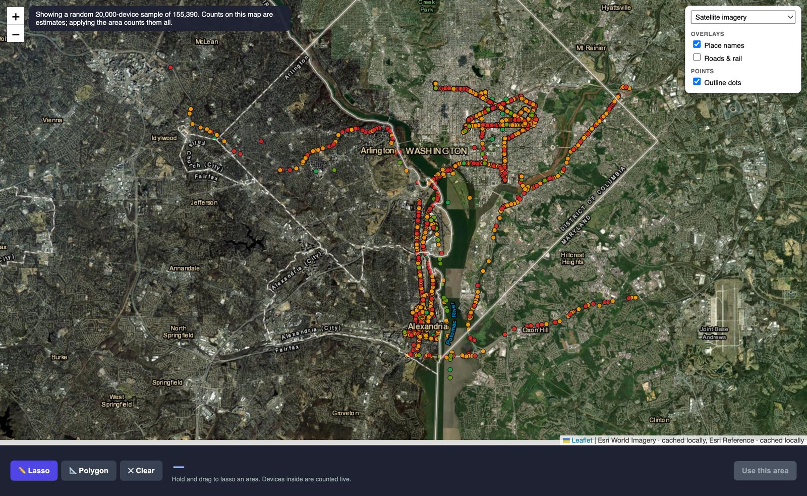
Above is one corpus in the area-selection view: a drive through Washington DC, Arlington and Alexandria. Every dot is an address, coloured by how strong its best sighting was, and they trace roads because that is where the car went. Draw a lasso and it counts what falls inside. That is the loop you actually spend your time in.

Note what the banner says. The map is holding a 20,000-point sample of 155,390 addresses, so it calls its own count an estimate rather than quietly reporting the number of dots it happens to have. That distinction is the whole subject of this page.

The number that shaped everything

A real corpus: 195 files, 9.1 million rows, 414,775 addresses.

Of those, 63% are rotating Bluetooth privacy addresses, which change every few minutes. Another 45% were seen exactly once, in one place. So the headline number is not a device count and never was — it is closer to a count of sightings that happened to carry a name.

The interesting question turned out to be geometric rather than statistical. For each address that is a durable identity, how far apart were its sightings and on how many separate days? That splits 145,507 durable identities into five groups, and the top one had nine members.

All nine were the operator's own kit. A watch, headphones, a phone, a pair of glasses.

That sounds like a disappointing result and it is the opposite of one. Tag those nine as yours, and the tenth arrival on that list is by definition something that travelled with you across days and countries and is not yours. Nine rows to check instead of four hundred thousand.

The useful output of a survey this size is not a list. It is a very short list, and an argument for why everything else was left off it.

Measure spread in kilometres, not grid cells

The first version counted how many map cells each address appeared in. Coarsen the grid from 0.1 degrees to 2 and the answer went 770, 17, 12, 9, then back up to 79 — not even monotonic, because an address sitting on a cell boundary gets counted twice and looks travelled.

Bounding-box diagonal in kilometres has no grid to be unlucky with. It returns exactly the nine that survived every cell size, and there is no knob to tune.

What broke

The map lied by a factor of eight. Large surveys get thinned before they are drawn, and the count was counting the dots it happened to be holding. Lasso an area and it reported 1,095 devices where the truth was 9,037. Worse, the thinning kept the strongest signals, so the colour ramp collapsed to solid green and the survivors clustered where the receiver had been close rather than where devices actually were. A uniform sample, scaled back to the true total and labelled an estimate, now reads within 2%.

"Random" and "rotating" are not the same thing. Bluetooth has three random address forms and only two of them change. Static-random addresses look anonymous but are fixed for the life of the device — they are the one random form you can follow. Calling them rotating told the operator that 34,557 devices were untrackable when they were the trackable ones. In the corpus they reappear in a later session 19.3% of the time against 5.2% for genuinely rotating ones.

The field that answers this cannot be trusted. Craxiom reports an address type per row, and the obvious move is to believe it. It labels 182,329 addresses PUBLIC whose bit pattern says otherwise — and those match a real IEEE vendor block just 1.6% of the time. A genuine public address is an IEEE assignment by definition, so that number should be near 100. Compare the rows it labels PUBLIC that also look public: 77.6% registry hits. Honouring the field would have declared 182,329 rotating addresses to be stable identities, which is a far larger error than the one being fixed, and every test in the suite would have sailed straight through it.

Half the discards were indoors, not lost. 709,470 rows had no GPS fix and were being thrown away. They were not scattered dropouts — the median gap was 27 minutes, which is a building, not a glitch. Anchoring each outage to the fixes either side recovered 641,002 of them, and every recovery site turned out to be an airport terminal. The other 68,044 stayed discarded, because the fix before and the fix after were hundreds of kilometres apart: that is a flight, and no position for it would be honest.

Sessions were being counted from filenames. The exporter rotates one mission across several files and writes Bluetooth, WiFi and LTE concurrently, so 12 actual missions looked like 185. Every "seen in N sessions" figure was inflated about 2.3 times until it started reading the mission id that was in every row all along.

Every bug worth finding here produced a plausible number rather than an error. Not one of them crashed anything. The suite has 392 tests and the ones that earn their keep are the ones that fail when you deliberately put the bug back — twice in this project a test named after a bug turned out not to detect it at all.

Why the counts are hedged everywhere

Device counts are substantially a measure of how long you stood still. Across ten sites visited on three or more days, the correlation between rows scanned and devices seen was 0.725, and the count varied ±48% between visits to the same place. So a raw total is never shown as a property of a place — it is shown next to the effort that produced it, and the durable-only figure, which is the one that actually compares.

The survey brief refuses to give a single distinct-device number too. It gives a range, and says which end to believe.

Areas you can use twice

A hand-drawn lasso is never reproducible. Two attempts at the same loading bay are different shapes, so counts from them cannot be compared. Saved zones keep the exact polygon, which is what turns "what changed here since last month" into a real question rather than an approximation.

Zones export to ATAK as Cursor-on-Target with the boundary travelling alongside the contacts — not just a scatter of pins with no way to see where the edge was, or to confirm on the next survey that you looked at the same ground. Contacts carry an honest error radius: a device positioned from an indoor anchor is not published as though it were a satellite fix.

Desktop only, and why

There is no browser demo. The tool reads other people's devices, and a public page with a working copy loaded against real data would be handing out both the instrument and a worked example on somebody's street. The screenshot above is a real survey; that is as much of one as belongs here.

The desktop version is the whole thing: parsing, the identity work, LTE tower positions from timing advance, co-travel detection, session diffing, saved zones, the CoT export, and a cache that turns a two-minute reprocess into thirteen seconds.